Counting, Heatmaps, and Speed Estimation

Three of the most common downstream pipelines — and the geometry behind them.

Most production computer vision systems aren't model.predict(). They're an object tracker plus a small piece of geometry: a line that objects cross, a polygon that defines a zone, a calibration that turns pixel velocity into meters per second. Build these once with Track mode and you can adapt them to almost any vertical.

Outcome

Implement line-crossing counting, zone occupancy, and a basic speed estimate from tracking output.

Fast Track

If you already know your way around, here's the short version.

Line crossing — track centroid moves from one side of a line to the other → +1.
Zone occupancy — point-in-polygon test on each tracked object → who's currently inside.
Speed — pixel displacement / time / pixels-per-meter → m/s.

Hands-on

Line-crossing counters

Conveyor belt packets counting with YOLO

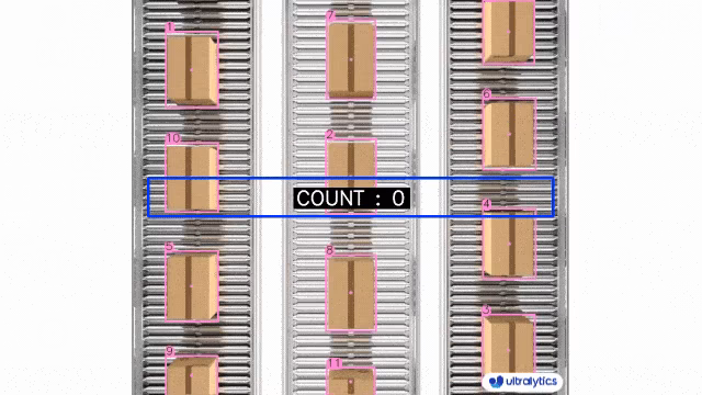
The simplest "people in / people out" counter. Define a line; count when an object's centroid crosses it.

from collections import defaultdict
from ultralytics import YOLO
from ultralytics.solutions import ObjectCounter

model = YOLO("yolo26n.pt")
counter = ObjectCounter(
    model="yolo26n.pt",
    region=[(20, 400), (1080, 400)],   # the line
    classes=[0, 2],                     # person and car only
    show=True,
)

for r in model.track("input.mp4", stream=True, persist=True):
    counter.process(r.orig_img)

print(f"In: {counter.in_count}, Out: {counter.out_count}")

The trick: a single line is a 2D segment. Direction is determined by which side of the line the track was on previously vs currently.

Zone occupancy

A polygon zone — count how many objects are inside it right now. The region counting guide ships a ready-made implementation if you'd rather not roll your own.

from shapely.geometry import Polygon, Point

zone = Polygon([(100, 100), (500, 100), (500, 400), (100, 400)])

for r in model.track("input.mp4", stream=True, persist=True):
    inside = 0
    for box in r.boxes:
        if box.id is None:
            continue
        x1, y1, x2, y2 = box.xyxy[0].tolist()
        cx, cy = (x1 + x2) / 2, (y1 + y2) / 2
        if zone.contains(Point(cx, cy)):
            inside += 1
    print(f"frame {r.path}: {inside} inside zone")

Speed estimation

Speed = pixel displacement between frames × calibration factor / frame interval. For real geographic scales, pair this with distance calculation.

The calibration factor (pixels-per-meter) depends on camera angle and is the messy part. Three options, in increasing accuracy:

Static field-of-view assumption — assume a known average ground-plane scale. Fine for rough speeds.
Marker calibration — measure a known length in the scene (a parking line, sign, lane width) and compute pixels per meter from it.
Homography — full 4-point ground-plane mapping. Most accurate; needed when the camera is angled.

from collections import defaultdict
from ultralytics import YOLO

model = YOLO("yolo26n.pt")
prev_centers: dict[int, tuple[float, float]] = {}
fps = 30
pixels_per_meter = 50    # measured: 50 px = 1 m on the ground plane

for r in model.track("input.mp4", stream=True, persist=True):
    for box in r.boxes:
        tid = int(box.id) if box.id is not None else None
        if tid is None:
            continue
        x1, y1, x2, y2 = box.xyxy[0].tolist()
        cx, cy = (x1 + x2) / 2, (y2)    # bottom-center is closer to ground plane
        if tid in prev_centers:
            px, py = prev_centers[tid]
            dx, dy = cx - px, cy - py
            dist_m = (dx ** 2 + dy ** 2) ** 0.5 / pixels_per_meter
            speed_ms = dist_m * fps
            print(f"track {tid}: {speed_ms:.1f} m/s")
        prev_centers[tid] = (cx, cy)

Use the bottom-center of the box, not the geometric center

The geometric center moves up when an object grows (gets closer to the camera). The bottom-center approximates the foot — which is on the ground plane. Speed estimates from bottom-center are far more stable.

Smoothing

Single-frame speed estimates are noisy. Average over a window:

from collections import deque

speed_window: dict[int, deque] = defaultdict(lambda: deque(maxlen=10))
# inside the loop:
speed_window[tid].append(speed_ms)
smoothed = sum(speed_window[tid]) / len(speed_window[tid])

A 10-frame window (~0.3s at 30fps) hides per-frame jitter without lagging too much.

Heatmaps

Heatmaps accumulate object positions over time into a 2D occupancy grid. Useful for spotting hot zones.

import numpy as np

heatmap = None
for r in model.track("input.mp4", stream=True, persist=True):
    h, w = r.orig_img.shape[:2]
    if heatmap is None:
        heatmap = np.zeros((h, w), dtype=np.float32)
    for box in r.boxes:
        x1, y1, x2, y2 = map(int, box.xyxy[0].tolist())
        heatmap[y1:y2, x1:x2] += 1

Visualize with a colormap or overlay on a static frame. Adjacent solutions like workouts monitoring and a Streamlit live inference UI use the exact same building blocks.

Try It

Implement a line-crossing counter for vehicles in any traffic video using the object counting helper or your own loop. Sanity-check the count against your eyes for a one-minute clip. The number should match within ±2.

Done When

You've finished the lesson when all of these are true.

You have a working line-crossing counter on a real video.
You understand why bottom-center is the right pixel for speed estimation.
You've computed a calibration factor (pixels per meter) for at least one scene.

What's next

One model, one stream — tractable. Many streams in parallel and the thread-safe inference discipline — that's the next lesson.

Get Started